Crystal Growth Simulator

CGSim package for analysis and optimization of Cz, LEC, and VCz growth of semiconductor crystals.

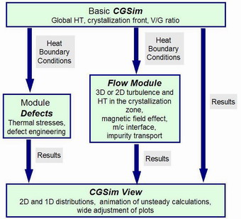Fig. 1. CGsim package.

Download printable version with application examples

The CGSim (Crystal Growth Simulator) code is specialized software for simulation of Czochralski (Cz), Liquid Encapsulated Czochralski (LEC), and Vapor Pressure Controlled Czochralski (VCz) growth. The code provides information to growers on the most important physical processes responsible for crystal growth and quality. The CGSim package contains several modules such as Basic CGSim, Defects, Flow Module, and CGSim View.

Basic CGSim

Capabilities of Basic CGSim include:

Radiative heat transport
Conductive heat transport
Heater power adjustment to provide the required crystallization rate
Calculation of crystallization front geometry
Automatic reconstruction of the geometry for several crystal positions
Special models for anisotropic characteristics of materials

The Basic CGSim program is developed for industries and research teams. Graphical User Interface of the Basic CGSim code requires no special computational skills. All setup and computational steps are highly automated to minimize user efforts.

Work with Basic CGSim includes the following stages:

Specification of the growth system geometry
Specification of material properties
Grid generation
Boundary condition specification
Problem mode specification
Computation process
Visualization of the results

Below, we will have a closer look at some of these stages.

Geometry Specification

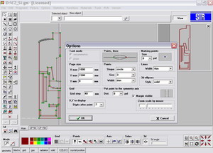Fig. 2. Specification of the Growth System in the Graphical User Interface (GUI)
The Basic CGSim has a convenient tool for geometry specification. Any geometry can be constructed by creating and manipulating geometric entities, such as, points, lines, curves, etc. To facilitate the geometry creation, the toolbox contains extensive set of tools for selecting, moving, splitting, connecting, and duplicating objects as well as tools for creating splines, polylines, and perpendiculars. If any modifications are introduced into the complex multiblock geometry, the user only needs to regenerate the grid and specify the materials in those blocks that were modified, while the rest of the setup stays intact.

Advanced users familiar with AutoCAD can use it as an alternative geometry specification tool and then import the geometry into CGSim using the DXF format.

The CGSim code is a software designed specially for 2D axisymmetrical computations, so the user only needs to create a half of the reactor geometry.

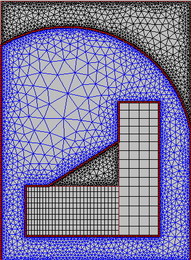
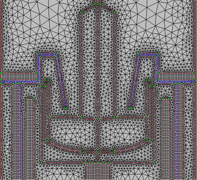
Grid Generation

The built-in geometry analyzer automatically recognizes closed contours as blocks, which substantially facilitates the geometry pre-treatment. This feature is also very useful as a diagnostics tool—if some area of the geometry, that stands for a separate construction element or a closed gas volume is not recognized as a block, it means that the contour representing its boundary is not closed. At the next step, the user can quickly generate a grid for the whole system using the auto grid generator. Since the automatic grid generator is very robust, the user only needs to set a parameter characterizing desired grid refinement to start the grid generation. GUI also provides the user with several options, facilitating the choice of blocks and grid types for the automatic grid generation. For instance, the user can choose the grid of some type to be generated in gas or solid blocks only.

Advanced users can customize the mesh manually in selected blocks or throughout the whole system. The grid generator supports triangular and quadrangular grids with both matched and mismatched interfaces. These capabilities are especially important for modeling of the crystallization front geometry, when structured grids are required on both sides of the interface. Local refinement of structured grids can be achieved through refining the node distribution on the respective edges towards one of the ends or symmetrically. For unstructured grids, refinement can also be regulated through the grid quality parameters.

Fig. 3. Examples of grids generated by Basic CGSim

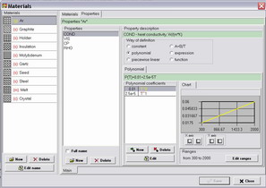
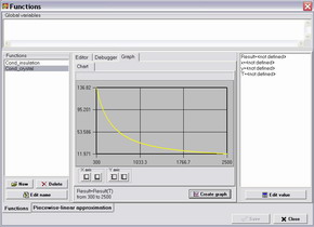
Materials

The CGSim tool for setting characteristics of materials gives the user wide possibilities. One can choose a constant, a polynomial function, a piecewise linear function, expression, or an arbitrary function, which can be programmed in the Function window. Plots for all characteristics can be displayed in the same window. For example, the heat conductivity can be defined as a function of temperature and coordinates in an arbitrary way borrowed from literature. Incorporated programming language similar to Pascal, extended by preprocessor and visualization of the function, allows this for user.

Fig. 4. Assigning the Material Properties in GUI

After the geometry creation and the material specification, Basic CGSim calculates the crystal and melt weights, and the initial charge weight, which helps the user to draw crystallization zone geometry. Beside the global heat computations with the given heater powers, Basic CGSim allows searching the powers providing a certain crystallization rate and prediction of crystallization front geometry.

The code permits automatic reconstruction of the geometry for several crystal positions. To make it, the user has to build only the geometry with the highest crystal position and to specify the crystal heights to be computed.

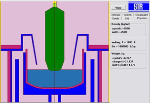Fig. 5. Crystal and Melt Weight Calculation

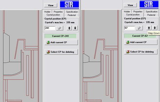Fig. 6. Automatic Reconstruction of the Crystal Positions

Module Defects

Module Defects is a part of the CGSim package specially designed for analysis of

thermal elastic stress distribution
behavior of initial defects such as self-interstitials and vacancies in silicon crystals
cluster distribution in silicon crystals (voids and oxygen precipitates).

Elastic Stress analysis

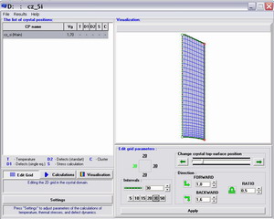Fig. 7. Module Defects Window
The elastic stress analysis is performed in the module in 2D axisymmetrical approximation. The numerical algorithm used in the module operates with the displacement vector u_i. The axisymmetric computational domain representing the crystal is meshed using cylindrical coordinates { r, j, z } with the temperature distribution found from the heat transfer modeling on the corresponding crystal position. The thermoelastic problem is solved using the Finite Volume Method. The following boundary conditions are used to solve the problem formulated above:

zero pressure is assigned along the crystal external boundary;
radial component of deformation vector u_r is equal to zero along the symmetry axis;
radial component of the force is equal to zero along the symmetry axis.

Several parameters can be used by the user to characterize strain-stress state in the crystal:

maximum s_max and minimum s_min principal stresses;
maximum shear stress s^sh_max which is critical for the gliding dislocation multiplication;
Von-Mises stress s_VM governing the change of crystal shape.

Simulation of initial defect incorporation

Initial lattice defects (single vacancies and self-interstitial atoms) are the sources for point defect clusterization during a crystal thermal treatment. Their concentrations determine the crystal quality to a large extent. The governing equation of initial defect incorporation into the crystal and their subsequent recombination in a hot region in vicinity of the crystallization front could be presented as
,
where C^eq_x is the equilibrium defect concentration and C_x is the actual defect concentration, D_x is the defect diffusivity, V is the crystal pulling rate, a_r is the recombination capture radius, and DG is the recombination free energy barrier (x = i, n for self-interstitials and vacancies, respectively).

Model of point defect clusterization

Certain characteristics of point defects formed during the crystal growth and subsequent wafer annealing are required for further making the integrated circuits (IC). Voids and oxygen precipitates near wafer surface can damage precise sub-micron IC elements. The model incorporated into the module accounts for simultaneous formation and evolution of voids and oxygen precipitates, allowing prediction of point defect concentrations and size distributions.

Flow Module

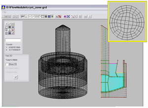Fig.8. Automatic 3D Grid Generation from the 2D Grid using octagonal blocks near the symmetry axis
Flow Module is desined for professional analysis of 3D or 2D turbulent and laminar convection in the crystallization zone including the melt, crystal, crucibles, and gas or encapsulant domains. A unique approach is used to couple this analysis with global heat transfer. The module allows the user to account for the following phenomena:

conductive heat transport;
laminar flow;
turbulent flow within the RANS, LES,or DNS approaches;
prediction of crystallization front shape;
magnetic field effect;
impurity transport;
stress computation;
scalar transport.

Automatic Generation of a 3D Grid

To provide grids for 3D computations, the Flow Module has an automatic 3D grid generator that builds 3D grids on the basis of 2D grids. Not only does it rotate the 2D grid around the vertical axis, but also incorporates blocks with quadragonal horizontal cross section in the central domains of the geometry, providing the area aroud the rotation axis with high-quality grid, see Fig. 8.

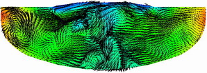
Turbulence models

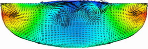
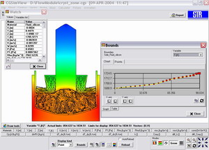Fig. 9. Flow pattern in the reactor and 1D temperature distribution along one of the boundaries
The user can choose the RANS, LES/URANS, DNS, or quasi DNS approaches and apply a model of turbulence specially adapted for the melt turbulent flow computations. Advanced approximations of convective and diffusive terms allow application of coarser computational grids and faster analysis. There are special tools for operative control of a computation.

Crystallization front geometry

Flow Module accurately describes the geometry of the crystallization front, temperature gradients, distributions of velocity vectors and scalars, heat and mass fluxes along interfaces. There are options to analyze unsteady effects in several monitoring points and in cross sections of a 3D grid. Parallel version of the solver is also developed for using on Linux clusters or on several PCs in a Windows network.

Magnetic field effects

Flow Module was extended by options for calculating magnetic field effects (MFs) in the crystallization zone, including the conjugated electric current flow in the crystal and melt]. There are automatic options for direct current magnetic fields of uniform (vertical or horizontal) and cusp configurations. Alternative current MFs can be implemented in a customized software version. Melt flow and the crystallization front can be analyzed in both 3D unsteady and 2D steady approaches. The examples on this page are provided for 400 mm diameter Si CZ growth.

Fig. 10. Temperature distribution and velocity distribution in the melt for 400 mm diameter Si CZ growth with zero magnetic field (left) and with horizontal magnetic field of 30 mT (right)

Solution control and visualization

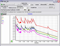
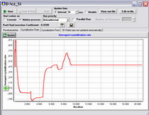
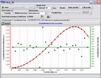
To control the computation execution, there is Computation Manager built-in into the program, which visualizes:

the equation residuals;
the averaged crystallization rate;
the crystallization front shape and the crystallization rate distribution along the melt-crystal interface;
distributions of the computed variables.

The computations are visualized with the CGSim Viewer program. Besides, it is possible to store a movie on a hard disk, showing the time behavior of the flow pattern.

Fig. 11. Monitoring of the Computation Progress

CGSim View

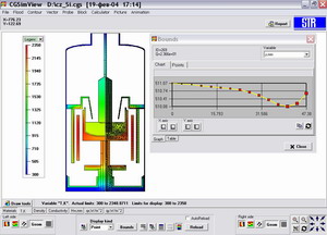Fig. 12. 1D and 2D Visualization with CGSim View
CGSim View allows analysis of 2D and 1D distributions including heat and mass fluxes, V/G ratio and temperature gradient along the crystallization front. Additionally, 1D distributions along a boundary can be displayed as a plot and stored in a file on a hard disk. Built-in animation tools help to analyze features of 3D melt convection.

Platforms

The present version of CGSim operates under Windows 2000 and Windows XP. The solver of Flow Module is available for parallel computations under Linux.

Additional information

Demo version and code documentation are available upon request.